From the Capital Asset Pricing Model to the Correlation Pricing Model

In the 1990s, when William Sharpe won the Nobel Memorial Prize for creating the capital asset pricing model (CAPM), the approach was an elegant way to break down stock returns to factors. CAPM is a single-factor model that links stock returns proportionally to their risk premiums. In other words, investors should adjust stock prices to a level that results in returns that proportionately compensate for the risk of owning those stocks. 

CAPM is very simplistic in nature and does not account for other risk or return premiums. This is where the Fama-French three-factor model later expanded CAPM by trying to explain stock returns using two additional factors (size and value). Since then, additional factors such as momentum and quality (profitability) have been proposed. Thus far, these additional factors tend to be characteristics of individual stocks.

As pioneers of smart beta—or, as WisdomTree prefers to call it, modern alpha—this company continuously researches existing and new factors. I have been writing about stock correlations acting as a precursor to heightened volatility. In my analysis below, I explain why correlations could be a key factor for persistent return premiums and information on market cycles.

Correlation Curves

Investors are familiar with term structure of interest rates—the yield curve. Each point on a curve represents an interest rate corresponding to a fixed duration of time plotted on the x-axis on a curve. 

A similar term structure could be plotted for average correlations for a given equity market. That is, each point of the curve would be the average of pairwise correlations between all stocks in an equity market for the corresponding trail back window of data on the x-axis.

Unlike interest rate term structures—where as you progressively go out, yields should be mostly higher due to a longer forward outlook and inflation expectations—our correlation curve should usually be flat. This is because in markets lacking systematic risk, the only difference between the calculation of near-term correlations (say, one month or three months) and far terms (say, 24 or 36 months) is simply additional trailing daily data. These average correlation numbers for longer windows should not be statistically different.

However, assets tend to be highly correlated during market corrections, so if there is a buildup of systematic risk, it usually manifests itself as near-term correlation values spiking up. This is evident in the table below, showing all three major financial crises over the last two decades: near-term correlations were higher than far-term correlations, causing the curve for S&P 500 stocks to follow what is known in the futures curve market as “backwardation.” 

If we exclude these crisis periods, the correlation curve was perfectly flat across the time periods shown. Spiking short-term correlations can thus be one warning sign of challenging times ahead. 

Consistency of Correlation Curve Signal 

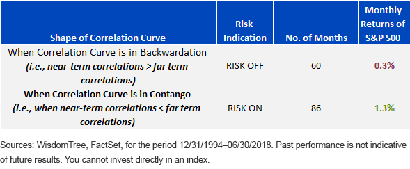
Next, to analyze the consistency and predictive ability of this correlation curve, I segregated the S&P 500’s average monthly performance in months immediately following two regimes:

1. Risk Off: When the correlation curve was in backwardation (downward sloping) or near-term correlations spiked¹

2. Risk On: When the correlation curve was in contango (upward sloping) or near-term correlations declined²

There was a substantial divergence in performance in the months following these signals. 

Not only did near-term correlations spike in crisis periods each time, but this also resulted in meaningful separation of performance in months that followed the spikes in correlations. To me, this correlation data thus carries meaningful information about stock behavior!

How Has the Correlation Curve Moved in 2018?

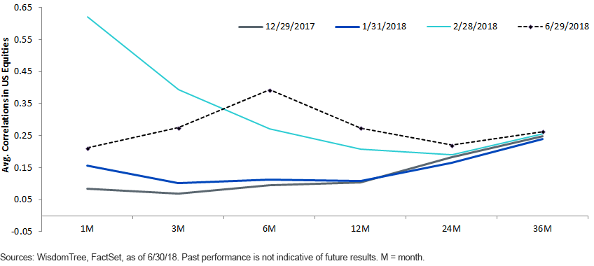
In January 2018, I noticed a pickup in this correlation curve compared with the December curve. This pickup was followed by a very sharp increase that continued in February, consistent with a massive spike in the Volatility Index on February 5, something that I covered in my blog post “What Do Rising Correlations Signal?”. Since then, near-term correlations have cooled, implying a sharp reduction in risk that was building up a few weeks earlier.

Spike in Near- Terms Average Correlations in 2018 Causing Backwardation in Correlation Term Strucuture

WisdomTree Solutions and Conclusions

As a leader of modern alpha strategies, WisdomTree constantly looks for factors that can help explain market behavior. When we launched our WisdomTree U.S. Multifactor Fund (USMF) in 2017 with an aim to provide multifactor exposure to the U.S. stocks, we used a combination of fundamental (value and quality) and technical (momentum and correlations) factors. The strategy aims to hold a basket of stocks that have the highest average score of all four factors, including correlations (stocks with low correlations having higher scores). While each of our factors adds value based on our proprietary methodology, correlation as a factor stands out: no other multifactor products currently offer a unique combination of correlation with the other more-common factors. 

WisdomTree is very pleased that our research is proving itself with since-inception returns of USMF better than most other popular multifactor strategies, something that our chief investment strategist recently covered in detail. 

In my opinion, correlation is a key piece of the factor puzzle: it can not only help explain how individual securities fit in a portfolio but also explain overall market behavior. On one hand, watching market correlations can give investors key insights into imminent market cycles; on the other hand, correlation as a factor combined with other factors can also help contribute to solid outperformance.

¹Curve was deemed to be in backwardation or downward sloping if nearest value (i.e., one-month average correlations) and farthest-out value (i.e., 36-month average correlation) are maximum and minimum, respectively, with an error or .05.
²Curve was deemed to be in contango or upward sloping if nearest value (i.e., one-month average correlations) and farthest-out value (i.e., 36-month average correlation) are minimum and maximum, respectively, with an error or .05.